Times: 9:00 AM – 2:00 PM (CST)
Location: Virtual
Instructor: Gordon Pierce, CDPHE Retired
Course Registration Link – Register by May 27, 2025
Who Should Attend: This course is specifically designed for regulatory air agency personnel who operate and oversee ambient air monitoring data. This class is intended for quality assurance coordinators or managers, field or laboratory supervisors, or technicians involved with quality assurance of monitoring system data.
Course Description: This course covers the basic design and theory of ambient air monitoring, quality assurance and control methods as they relate to monitoring instruments, site development criteria and data processing. This course will address PM2.5 and other particulate methods, ozone, oxides of nitrogen, carbon monoxide, hydrocarbon, sulfur dioxide, meteorology systems, data recording systems, gas calibration systems, and zero air systems.
Learning Objectives: Those completing this course will gain a basic understanding of the general information associated with principles of ambient air monitoring. Attendees will be able to perform regulatory reviews involving the following elements of ambient air monitoring:
- Regulations and Standards
- Monitoring Networks
- Station Siting
- Instrumentation
- Documentation
- Data Handling
- Quality Assurance
- References and Resources
Course Delivery: This is a virtual instructor-led training that will use an online webinar platform to deliver the material. The instructor will use engagement exercises, such as online polls or breakout rooms, to help keep the participants’ attention during the two 1/2 day sessions.
Agenda
| Times (Central) | Subject |
|---|---|
| Day 1 | |
| 9:00 | Introduction/Course Overview |
| 9:30 | Regulations and Standards |
| 10:00 | Monitoring Networks |
| 10:30 | Break |
| 10:45 | Monitoring Networks (con’t) |
| 11:15 | Station Siting |
| 12:00 | Lunch |
| 1:00 | Measurement Process |
| 1:45 | Q & A |
| 2:00 | Adjourn (End of Day 1) |
| Day 2 | |
| 9:00 | Review of Day 1 |
| 9:15 | Measurement Process (Con’t) |
| 10:00 | Data Handling |
| 10:30 | Break |
| 10:45 | Documentation |
| 11:15 | Quality Assurance/Quality Control |
| 11:45 | References and Resources |
| 12:00 | Q & A |
| 12:30 | Adjourn (End of Day 2) |
Questions?
Instructor Contact: Gordon Pierce (glpierce87@att.net)
Training Coordinator: Zac Adelman (adelman@ladco.org)
Accessibility Statement
LADCO strives to host inclusive, accessible training events that enable all individuals, including individuals with disabilities, to engage fully with the instructor and course content. To request an accommodation or for inquiries about accessibility, please contact Zac Adelman (adelman@ladco.org | 847-720-7880).
]]>App Description
The LADCO Urban Increment R-Shiny App displays the urban, rural, and urban increment PM2.5 concentrations for urban areas across the lower 48 states. Users can select one or more states, and then one or more urban areas in the selected states to display a stacked bar chart and tabulated urban increment data. Descriptions of the data and methods used to develop this tool follow.
Background
With the promulgation of a revised annual PM2.5 standard in February 2024 there is a demand for new air quality analysis products to understand the current profile of particulate pollution in the U.S. One of the data analysis products that contributes to the nonattainment area designations process is an urban increment analysis (see section 1.4 of US EPA, 2024). Per this memo, “the goal of the urban increment analysis is to estimate the local contribution to urban PM2.5 as measured at violating regulatory monitor sites and thereby provide additional evidence to consider in deciding which nearby areas with sources contributing to the monitored violations in the area to include within the boundary of the designated nonattainment area.”
The conventional approach for an urban increment analysis is to use surface monitors cited in urban and rural areas to estimate an urban increment at potential violating monitors. The urban monitors are part of the Chemical Speciation Network (CSN), and the rural PM2.5 concentrations are estimated using data from the IMPROVE program. The urban increment is simply the difference between a period-averaged concentration at the urban monitor and an analogous concentration at rural monitors that are within 150 miles of the urban site. Given the sparsity of the IMPROVE network, particularly in the Great Lakes region, there is an opportunity to explore alternative urban increment analyses that are based on PM2.5 data with more continuous spatial coverage.
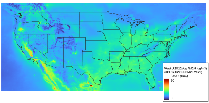
Satellite PM2.5 Data
The Atmospheric Composition and Analysis Group at Washington University have developed satellite-derived global and regional PM2.5 data. These data are a fusion of satellite, modeled, and surface data. The fused data are estimated for “annual and monthly ground-level fine particulate matter (PM2.5) by combining Aerosol Optical Depth (AOD) retrievals from the NASA MODIS, MISR, SeaWIFS, and VIIRS with the GEOS-Chem chemical transport model, and subsequently calibrating to global ground-based observations using a residual Convolutional Neural Network (CNN).” The V6.GL.02.02 data are available for 1998-2022 on a 0.01 degree grid. Given the spatial continuity of these data and their relatively high correlation with surface observations, they provide a viable alternative to surface monitors for use in an urban increment analysis.
Methods
I used a GIS (QGIS 3.24.0) to conduct all of the calculations and data processing steps for this analysis. The basic approach was to convert the netCDF gridded PM2.5 data to a raster, clip the PM2.5 data by urban and rural landuse, and then use zonal statistics to get the average concentrations in the rural and urban areas of each state. With the urban and rural concentrations I could then calculate the urban increment in each urban area. Here are the detailed steps and data that I used.
Data
- PM2.5 data: 2022 global 0.01 degree PM2.5 data in netCDF format (Washington University V6.GL.02.02)
- State boundaries: 2016 state boundary shapefile (US Census @ 1:500,000)
- Urban areas: 2023 urban area shapefile (US Census Tiger Line)
Processing Steps
- Use R to convert netCDF PM2.5 data to a raster and window in on the U.S. (download R code).
- Load the PM2.5 raster and the two shapefiles above into QGIS.
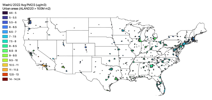
- Filter the urban area shapefile to include only medium and larger cities. I used the land area (ALAND20) attribute to Extract by expression only urban polygons with land areas greater than 100 million m2.
- Clip the Air Pollution Raster by the Urban Land Use
- Vectorize the Urban Areas:
- Use the Rasterize (vector to raster) tool to create a binary raster that represents urban areas. The resulting raster will have values of 1 for urban areas and “no data” for non-urban areas. Use the filtered urban shapefile from step 3 above.
- Vectorize the Urban Areas:
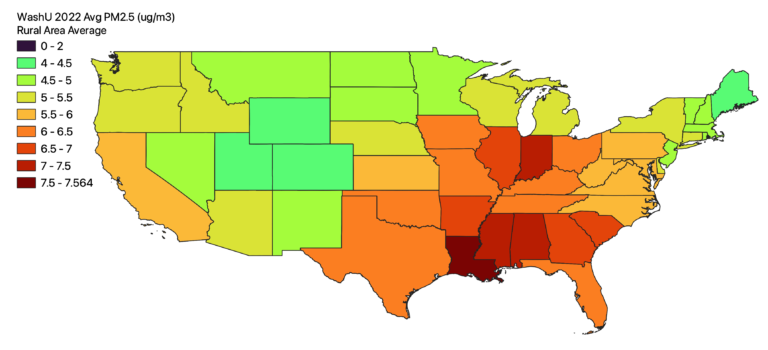
- Mask the air pollution data to the non-urban (rural areas):
- Use the Fill NoData cells tool to replace the “no data” values in the binary urban raster from above with “0”.
- Use Raster Calculator to invert the urban raster to create a non-urban raster by subtracting the updated binary urban raster from 1, e.g., “1 – urban”. The resulting raster file will have “1” for the non-urban areas on “0” for the urban areas.
- Use Raster Calculator to multiply the air pollution raster by the binary non-urban raster. This will mask the air pollution data to only non-urban areas. This is the intermediate dataset that will be used to calculate the rural PM2.5 concentrations in each state.
- Calculate the urban and rural concentrations in each state:
- Zonal Statistics by Urban Area:
- Open the Zonal Statistics tool (
Raster→Zonal Statistics). Choose the filtered urban area boundary shapefile as the vector layer. - Select the rasterized netCDF air pollution file (created in step 1) as the raster layer.
- Set the statistic type to calculate (mean, sum, etc.). For average concentration, select the mean.
- Run the tool, which will add a new attribute to your urban shapefile containing the mean PM2.5 air pollution concentration for each urban area
- Open the Zonal Statistics tool (
- Zonal Statistics by Rural Area:
- Open the Zonal Statistics tool (
Raster→Zonal Statistics). Choose the state boundary shapefile as the vector layer. - Select the non-urban PM2.5 raster (created in step 5) as the raster layer.
- Set the statistic type to calculate (mean, sum, etc.). For average concentration, select the mean.
- Run the tool, which will add a new attribute to your state shapefile containing the mean rural PM2.5 concentration for each state
- Open the Zonal Statistics tool (
- Zonal Statistics by Urban Area:
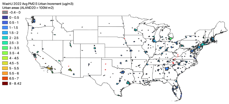
- Combine all of the data into a single shapefile and calculate the urban increment
- Add state attributes to the urban area shapefile
- Because the urban area feature from the Census doesn’t have a state ID, add it in using the Join attributes by location tool. You can directly join the augmented state shapefile with rural concentrations from the previous step since it has all of the information we’ll need here.
- Start with the urban shapefile that includes the mean PM2.5 concentrations created in step 6, and Join attributes by location selecting the state shapefile with rural concentrations as the layer to join with. For the geometric predicate select “intersect” and for the Join type “take attributes from the feature with the largest overlap”. This last step ensures that for multi-state urban areas we will associate with the rural concentration from the state that most intersects with the urban polygon.
- Calculate the urban increment
- Use the field calculator to take the difference of the urban mean concentration and the state rural mean concentration to get the urban increment for each urban area
- Output the new Shapefile with the state and urban metadata, the urban PM2.5 concentrations, rural PM2.5 concentrations, and urban PM2.5 increment.
- Add state attributes to the urban area shapefile
Results
Wednesday July 24, 2024 @ 11:00 – noon Central (Teams Link)
Victor Geiser, LADCO Summer-2024 Intern

Abstract: In this study, we used Self Organizing Maps (SOMs) for analyzing the meteorological conditions during June days from 2019 through 2023 and associated PM2.5 concentrations in the Midwest. Through an understanding of synoptic scale meteorological patterns and an introspective look at the vertical structure of the atmosphere, we gauge common and less common weather patterns for various levels of PM2.5 concentrations including those influenced significantly by wildfire smoke transported into the LADCO region.
The figure below shows the daily fine particle pollution (PM2.5) concentrations average across all monitors in the Great Lakes region for the year 2019-2023. Each colored line represents the daily average for each year. The particle concentrations in 2023 are shown by the blue line, with several high pollution events between June and September. The late June 2023 event was historic and led some media outlets to declare that cities in the region had the “worst air pollution in the world” during that period.

LADCO supports air quality planners in the region
LADCO works with our member states to track and understand the impacts of fire smoke on air quality in the region. Wildfire smoke poses a challenge for state and local air quality planning agencies in the Great Lakes region because it falls outside of their regulatory jurisdictions. There is nothing a state planning agency can do about controlling pollution from fire smoke, particularly if the fires are located far away, like Canada or the western U.S.
LADCO uses data science and computer modeling to quantify the amount of pollution entering the region from wildfires, and to identify the days during which smoke-influenced pollution is the worst. We work with our member states and U.S. EPA to account for pollution periods caused by transported wildfire smoke.
LADCO in the news discussing fire smoke and air quality
LADCO’s Executive Director has been in the news quite a bit since summer 2023 talking about wildfire smoke and air quality in Chicago.
The health of effects of Chicago’s Air Pollution (NPR, July 11, 2023)
Smoke from large wildfires can spread wide and far. In 2018 we observed smoke on several days in the LADCO region that originated from fires in the western U.S. and Canada. Wildfire smoke is a concern because it contains harmful air pollutants, including particles, air toxics, and ozone precursors [1,2]. The health impacts from fire smoke exposure include increased rates of respiratory diseases, such as asthma and chronic obstructive pulmonary disease.
The image above shows wildfire smoke viewed from space on August 4, 2018. Darker shades of grey indicate thicker layers of smoke. The circles overlaid on this plot are daily maximum ozone concentrations at monitoring sites. Orange and red colors represent locations with unhealthy air quality concentrations. This image of smoke impacts is fairly typical of the summer of 2018, in which large fire complexes in the Western U.S. produced smoke that blanketed the atmosphere over the majority of the country.
Smoke that is transported into the LADCO region degrades our air quality. Ozone, fine particulate matter, and regional haze may all be influenced by smoke that originates from thousands of miles away. LADCO is working with our member states to understand the trends in smoke impacts on our region and what the implication of these impacts are on public health and regulatory compliance. We are integrating surface monitoring, remote sensing, and modeling into a data platform to identify in near real-time the extent to which fire smoke is exacerbating air pollution in our region.
]]>